Survival Analysis Models

Survival analysis is a statistical method used to modeling object behavior dependent on set of variables (x1 .. xn) in time-to-event period. It is especially useful in modeling the probability of object’s survival in certain circumstances. One can analyze a timeline to events occurrences in relation to variables influencing the time until a specific event occurs like death, failure, or customer say “Goodby to the company”. Here’s a breakdown of key terminology of survival analysis.

Key terminology of survival analysis models

• Event: The outcome of interest, such as death, disease occurrence, customer churn, or equipment failure.
• Time: The duration from a defined starting point (e.g., start of treatment or customer acquisition) to the occurrence of the event or the end of observation (censoring).
• Censoring: When the event of interest is not observed for some individuals during the study period, making their exact survival time unknown.
• Survival Function S(t): The survival function S(t) is defined as the probability that a subject survives (i.e., does not experience the event) beyond time t.
• Hazard Function h(t): The hazard function h(t) represents the instantaneous rate at which the event occurs at time t, given that the subject has survived up to that time.
• Linking the Survival and Hazard Functions: The survival and hazard functions are mathematically related. Knowing one allows you to derive the other, reflecting the duality between retention (survival) and churn (event occurrence).

Linking the Survival and Hazard Functions

The survival and hazard functions are mathematically related. Knowing one allows you to derive the other, reflecting the duality between retention (survival) and churn (event occurrence).

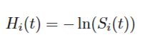
In summary, the cumulative hazard rate of subject i at time t can also be defined as the negative logarithm of the survival function at time t.

Stratification

When we have a variable influence in some moment of time, we can divide the period of observation to two periods, when the time before the variable application and the the time post. It constitutes a new starting point of the new treatment application to the patient. The shift of the survival function could be observed.

Kaplan-Meier Estimator

Kaplan-Meier Estimator is a non-parametric model for estimating the survival function, often used as a first step in survival analysis. It demonstrate the probability of survival a certain time in function of time. The maximum value is 1 and the K-M curve goes approximately to zero when time increases.

Cox Proportional Hazards Model

Cox Proportional Hazards Model is a semi-parametric model that incorporate the influence of some predictor variables to the hazard rate or survival model.  Each subject has an observed survival time 0-t and an event variable xE that shows whether the event has occurred. It is also observed in time 0-t tat variables x1 .. n have had an influence on event xE occurrence. The Cox model incorporate the influence of x1 .. xn factors to estimation the time of survival or hazard rate as n explanatory variables. This make the model can also predict a time of survival.

Disclaimer: the post is inspired by: Benjamin Lee, A Comparison Study of Parametric and Machine Learning Survival Analysis Models to Predict Customer Churn in the Edtech Sector, Vienna, 27th January, 2025
Benjamin Lee, Peter Filzmoser, link: here

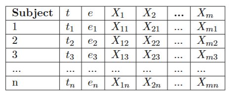
Dataset for Cox Proportional Hazards Model

If we have dataset like here

The Kaplan-Meier estimator is the statistical tool used to estimate a true survival function from available data and can be considered the ’best’ estimator of survival probability when no parametric structure is assumed. This estimator is a non-parametric estimator that only requires the time-to-event (or time-to-censoring) t , and the event status e for every subject. With this information, the survival function estimator S(t) is given by:

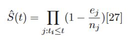
where e_j is the time at which at least one event e occurred, and n_j is the total number of subjects who have been censored or have not had the event yet at time t_j .

One of the main drawbacks of the Kaplan-Meier model is that it is not able to take any subject covariates into account – what means, it does not provide explanatory power in terms of different variables within a group.

Understanding the Cox Proportional Hazards Model

When we want to understand how factors like age, treatment type, or blood pressure affect survival time, the Cox Proportional Hazards model is a go-to tool. Instead of trying to pin down the exact risk at every single moment, this model cleverly separates the hazard rate into two distinct parts.

The core idea is to model how specific factors (or covariates) have a multiplicative effect on an underlying hazard rate. The formula for the model looks like this:

h(t,X)=h₀​(t)⋅exp(βX)

Let’s break that down:

• h_0​(t) is the Baseline Hazard. Think of this as the underlying risk of the event for a “standard” individual (where all covariate values are zero) over time. It’s the part of the model that changes with time (t), but it’s “non-parametric,” meaning we don’t assume its shape. We let the data speak for itself.
• exp(βX) is the Covariate Effect. This is the parametric part of the model and it’s where your specific factors come in.
  • X is the set of your covariates (e.g., age, treatment type, or blood pressure).
  • β are the coefficients, similar to those in a linear regression, that the model estimates.
  • This component tells us how much an individual’s unique characteristics increase or decrease their risk compared to the baseline. Applying the exponential function, exp(), ensures this multiplier is always positive, as negative risk doesn’t make sense.

Notice that only the baseline hazard depends on time. The covariate effect, exp(βX), is constant over time. This separation is the key to the model’s power and leads directly to its most important assumption.

---

In the Cox proportional hazards model, a covariate is a predictor variable that you include in the model to explain or predict the risk (hazard) of a specific event occurring over time, such as death, failure, or relapse. These covariates can be continuous (e.g., age, blood pressure) or categorical (e.g., treatment group, gender).

What the program calculates:

• The model estimates the effect of each covariate on the hazard function—the instantaneous risk of the event happening at a certain time.
• It computes coefficients (often denoted as ββ) for each covariate, quantifying how the risk changes with a one-unit increase in that variable, assuming other covariates remain constant.
• These coefficients translate into hazard ratios (exponentiated coefficients), which tell how much the hazard (risk) is multiplied by when the covariate changes by one unit.
• The baseline hazard function h0(t)h0(t) represents the hazard if all covariates were zero; the model then scales this baseline hazard depending on the values of the covariates for each individual.
• Overall, the Cox model evaluates how your covariates modify the risk of the event over survival time, assuming that these effects multiply the baseline hazard proportionally and do not change with time (proportional hazards assumption).

Formally, the hazard function is modeled as

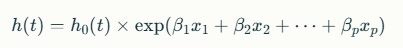
where x1,x2,…,xpx1,x2,…,xp are your covariates and β1,β2,…,βpβ1,β2,…,βp are their estimated effects.

Summary:

• Your covariate is any variable in your data that may affect the timing of the event.
• The Cox model calculates how these covariates affect the hazard or instantaneous risk of the event happening, summarized through hazard ratios.
• This helps you understand which factors increase or decrease risk while accounting for the survival time and censoring in your dataset.

This explanation aligns with standard survival analysis literature and is consistent with how lifelines or R coxph functions use covariates in the Cox model.

The “Proportional” in Proportional Hazards

The model’s name comes from its core assumption: the effect of the covariates is constant over time. In other words, the hazard ratio between any two individuals remains proportional throughout the entire timeline.

Let’s make this concrete. Imagine we have a single covariate, x – age, and two subjects, ‘a’ and ‘b’. Their hazard rates are:

• Subject a: h(t,x_a​)=h_0​(t)⋅exp(βx_a​)
• Subject b: h(t,x_b​)=h₀​(t)⋅exp(βx_b​)

If we look at the ratio of their hazards, the baseline hazard h₀​(t) cancels out:

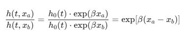
As you can see, time (t) has vanished from the right side of the equation. This means that if subject ‘a’ has double the risk of subject ‘b’ on day 1, they will also have double the risk on day 100 or day 500. The risk difference is because of age difference. Their relative risk is constant, or proportional. This powerful assumption is a direct consequence of the model’s structure.

If one has a dataset which violates the proportional hazards assumption, it causes reduction in predictive power of the model. The hazard as an output from the model is a useful tool in assessing the general magnitude of a covariates’ effect on the time of survival. One can interpret the hazard ratio as the weighted average of true hazard ratios over the time period. Therefore, one must not strictly conform to the proportional hazards assumption, but always check if dataset is appropriate to this assumption.

You can check if your dataset meets the proportional hazards assumption of the Cox model using both visual plots and formal statistical tests.

---

Visual Inspection (Graphical Methods)

Visual checks are often the first and most intuitive step.

Log-Log Survival Plots

This is a classic method for categorical covariates (like “treatment group” vs. “control group”).

• How it works: You plot the logarithm of time, log(t), on the x-axis against a special transformation of the survival probability, -log(-log(S(t))), on the y-axis for each group.
• What to look for: If the proportional hazards assumption holds, the resulting curves for each group should be roughly parallel and not cross. If the lines cross or move closer or further apart in a systematic way, the assumption may be violated.

Schoenfeld Residuals Plots

This is the most common and powerful visual method, and it works for both continuous and categorical covariates.

• How it works: For each event that occurs, a residual is calculated that represents the difference between the observed covariate value and the expected covariate value for the individual who had the event. You then plot these residuals against time.
• What to look for: If the assumption holds, you should see a random scatter of points around a horizontal line at zero. If you see any clear pattern or trend (e.g., a line with a positive or negative slope), it suggests the effect of the covariate changes over time, violating the assumption.

---

Formal Statistical Tests

A formal test gives you a p-value to help you decide if any violations you see are statistically significant.

• How it works: The most common test is based on the Schoenfeld residuals. It formally tests whether the slope of a line fitted to the Schoenfeld residuals-vs-time plot is significantly different from zero. This is often done using a function like cox.zph() in R or the check_assumptions() method in Python’s lifelines library.
• How to interpret the results:
  • Null Hypothesis (H_0): The effect of the covariate is constant over time (the proportional hazards assumption holds).
  • A low p-value (e.g., < 0.05) suggests you should reject the null hypothesis. This is evidence that the assumption is violated for that specific covariate.
  • A high p-value means you fail to reject the null hypothesis, so it’s reasonable to assume the proportional hazards assumption is met.

---

Example of check_assumptions(data) in Python

The dataset includes:

• Subject ID
• Survival time in days
• Event status (1 = event occurred, 0 = censored)
• Age group (1 – 4)

To use check_assumptions() from lifelines, you need to fit a Cox Proportional Hazards model, which requires at least one covariate (a variable that might affect survival, ex age group).

from lifelines import CoxPHFitter

# Fit the Cox model
cph = CoxPHFitter()
cph.fit(data, duration_col="Survival_in_days", event_col="Status_bool")

# Check proportional hazards assumption
cph.check_assumptions(data)
# or
cph.check_assumptions(data, p_value_threshold=0.05)

What to Do If the Assumption is Violated

If you find that a key variable violates the assumption, you have options:

1. Stratification: You can stratify your model by the problematic covariate. This allows the baseline hazard function to be different for each level of that variable, resolving the violation. For example, if “gender” violates the assumption, you can stratify by it.
2. Use Time-Dependent Covariates: You can modify the model to include an interaction term between the covariate and time. This explicitly models how the covariate’s effect changes over time.
3. Choose a Different Model: If the violation is severe, a parametric model (like a Weibull or Log-Logistic model) that has a built-in shape for the hazard function might be a more appropriate choice for your data.

Parametric Models

When the underlying probability distribution of the dataset is known, one can use parametric models to model the survival function of the dataset. Once the underlying model is specified either in terms of the survival times or the logarithm of survival times, the model can be fitted and estimated using the maximum likelihood estimator.

Of course. Parametric models in survival analysis assume that a subject’s survival time follows a specific, known statistical distribution (like the exponential or Weibull distribution). Unlike non-parametric models (e.g., Kaplan-Meier) which don’t make assumptions about the data’s distribution, parametric models are defined by a set of parameters that dictate the shape of the survival and hazard functions.

Understanding them means understanding the hazard function each model assumes. The hazard function describes the instantaneous risk of an event occurring at a specific time, given that it hasn’t occurred yet.

---

Exponential Model

This is the simplest parametric model. It assumes the hazard rate is constant over time.

• Core Idea: The risk of the event happening is the same every single day. If a component hasn’t failed by day 10, its risk of failing on day 11 is the same as it was on day 2.
• Hazard Function: h(t)=λ (a constant)
• How to Understand It: This model is defined by a single parameter, λ (lambda), the hazard rate. It’s best suited for events that don’t have a “memory” or aging process, such as the failure rate of certain electronic components or the occurrence of random external events.

Weibull Model

The Weibull model is a more flexible and widely used model because it does not assume a constant hazard rate.

• Core Idea: The risk of the event can increase, decrease, or remain constant over time. This makes it much more adaptable to real-world scenarios.
• Hazard Function: h(t)=λk(λt)k−1
• How to Understand It: The model is defined by two main parameters:
  • λ (scale parameter): Stretches or compresses the curve.
  • k (shape parameter): This is the key. It dictates the nature of the hazard.
    • If k>1, the hazard increases over time (e.g., aging, where the risk of failure grows).
    • If k<1, the hazard decreases over time (e.g., post-surgery recovery, where the initial risk is high but drops).
    • If k=1, the Weibull model simplifies to the Exponential model with a constant hazard.

Log-Normal and Log-Logistic Models

These models are useful for situations where the hazard rate is not monotonic (i.e., it doesn’t just go up or down).

• Log-Normal Model
  • Core Idea: Assumes that the logarithm of the survival time follows a normal (bell-shaped) distribution.
  • Hazard Function: The hazard rate first increases to a peak and then decreases.
  • How to Understand It: Think of situations where failure is most likely after a certain “wear-in” period, but if the subject survives past that peak, the immediate risk then declines. It’s often used in engineering for component fatigue.
• Log-Logistic Model
  • Core Idea: Similar to the Log-Normal model, it also assumes the logarithm of survival time follows a specific distribution (the logistic distribution).
  • Hazard Function: The hazard rate can be hump-shaped (increasing then decreasing) or monotonically decreasing, depending on its parameters. It’s more flexible than the Log-Normal model.
  • How to Understand It: This model is popular in medical research, especially when studying diseases like cancer where the risk of mortality might peak some time after diagnosis and then fall. It’s also notable because its survival function has a simple, explicit formula, which makes interpreting odds easier.

Accelerated Failure Time (AFT) models

In contrast to the Cox model, AFT models assume that covariates are proportional with respect to survival time.

Metrics for Survival Analysis

Log-Rank Test

The log-rank test is used to compare two or more survival functions with each other. In this sense, it is analogous to the t-test or Pearson’s chi-squared test for survival analysis. Like those tests, the log-rank test tests the null hypothesis H0 that there is no difference between the survival functions being compared in the probability of an event e occurring at any time t.

The Log-Rank Test is a statistical test used in survival analysis to compare the survival distributions of two or more groups. It’s particularly useful for determining if there are significant differences in the time it takes for an event (like death, failure, or relapse) to occur between groups.

Example Calculation

Let’s consider a clinical trial comparing the survival times of patients using two different cancer treatments, Drug A and Drug B. Here’s a simplified dataset:

Time (months)	Event (1=death, 0=censored)	Group (A/B)
2	1	A
3	0	A
4	1	B
6	1	A
7	0	B
8	1	B

Steps to Calculate the Log-Rank Test:

1. Combine the Data: List all unique time points from both groups.
2. Calculate the Number at Risk: For each time point, determine how many patients are still at risk in each group.
3. Calculate the Expected Events: For each time point, calculate the expected number of events (deaths) for each group.
4. Compute the Test Statistic: Use the observed and expected events to calculate the test statistic.

Detailed Calculation:

1. Combine the Data:
   • Time points: 2, 3, 4, 6, 7, 8
2. Number at Risk:
   • At time 2: Group A: 2, Group B: 3
   • At time 3: Group A: 1, Group B: 3
   • At time 4: Group A: 1, Group B: 2
   • At time 6: Group A: 1, Group B: 2
   • At time 7: Group A: 0, Group B: 2
   • At time 8: Group A: 0, Group B: 1
3. Expected Events:
   • At time 2: Expected events for Group A = (2/5) * 1 = 0.4, Group B = (3/5) * 1 = 0.6
   • At time 4: Expected events for Group A = (1/3) * 1 = 0.33, Group B = (2/3) * 1 = 0.67
   • At time 6: Expected events for Group A = (1/3) * 1 = 0.33, Group B = (2/3) * 1 = 0.67
   • At time 8: Expected events for Group A = 0, Group B = 1
4. Test Statistic:
   • Sum the observed and expected events for each group.
   • Calculate the test statistic using the formula:
   $ \chi^2 = \sum \frac{(Oi – Ei)^2}{E_i} $ Where ( Oi ) is the observed number of events and ( Ei ) is the expected number of events. For our example, the test statistic would be calculated based on the observed and expected events at each time point.

If the test statistic is greater than the critical value from the chi-square distribution table (with 1 degree of freedom), we reject the null hypothesis and conclude that there is a significant difference between the survival distributions of the two groups [1] [2].

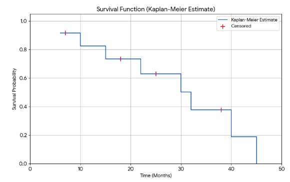
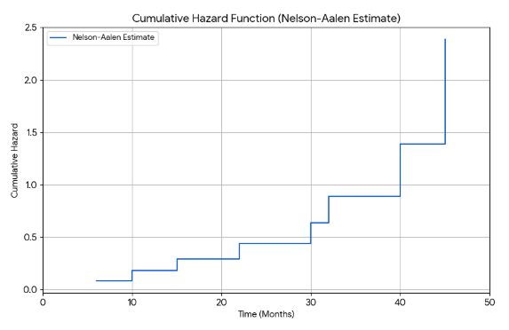
Example of Survival Analysis Models in Python

The code demonstrate a plot of survival and hazard functions.

import pandas as pd
import numpy as np
import matplotlib.pyplot as plt

# --- 1. Create a Sample Dataset ---
data_dict = {
    'time': [6, 7, 10, 15, 18, 22, 25, 30, 32, 38, 40, 45],
    'event': [1, 0, 1, 1, 0, 1, 0, 1, 1, 0, 1, 1]  # 1 = event, 0 = censored
}
data = pd.DataFrame(data_dict)
data = data.sort_values(by='time').reset_index(drop=True)

# --- 2. Calculate Kaplan-Meier Survival Function ---
km_data = data.copy()
unique_times = sorted(km_data['time'].unique())
survival_prob = 1.0
results = []

for t in unique_times:
    at_risk = (km_data['time'] >= t).sum()
    events = km_data[(km_data['time'] == t) & (km_data['event'] == 1)].shape[0]
    
    if at_risk > 0:
        survival_prob *= (1 - events / at_risk)
    
    results.append({'time': t, 'survival': survival_prob})

km_results = pd.DataFrame(results)

# --- 3. Plot the Survival Function ---
plt.figure(figsize=(10, 6))
plt.step(km_results['time'], km_results['survival'], where='post', label='Kaplan-Meier Estimate')
plt.scatter(data[data['event'] == 0]['time'], km_results.loc[data[data['event']==0].index, 'survival'],
            marker='+', color='red', s=100, label='Censored')
plt.title('Survival Function (Kaplan-Meier Estimate)')
plt.xlabel('Time (Months)')
plt.ylabel('Survival Probability')
plt.ylim(0, 1.05)
plt.xlim(0, max(data['time']) + 5)
plt.grid(True)
plt.legend()
plt.savefig('manual_survival_function_plot.png')
plt.close()

# --- 4. Calculate Nelson-Aalen Cumulative Hazard ---
na_data = data.copy()
hazard = 0.0
na_results_list = []

for t in unique_times:
    at_risk = (na_data['time'] >= t).sum()
    events = na_data[(na_data['time'] == t) & (na_data['event'] == 1)].shape[0]

    if at_risk > 0:
        hazard += events / at_risk
    
    na_results_list.append({'time': t, 'cumulative_hazard': hazard})

na_results = pd.DataFrame(na_results_list)

# --- 5. Plot the Cumulative Hazard Function ---
plt.figure(figsize=(10, 6))
plt.step(na_results['time'], na_results['cumulative_hazard'], where='post', label='Nelson-Aalen Estimate')
plt.title('Cumulative Hazard Function (Nelson-Aalen Estimate)')
plt.xlabel('Time (Months)')
plt.ylabel('Cumulative Hazard')
plt.xlim(0, max(data['time']) + 5)
plt.grid(True)
plt.legend()
plt.savefig('manual_cumulative_hazard_plot.png')
plt.close()

[1]: DATAtab [2]: Real Statistics Using Excel

References

[1] Log-Rank Test: A Beginner’s Guide – DATAtab

[2] Log-Rank Test – Real Statistics Using Excel