Moving average in SQL
The post will explore two methods for creating a moving average in SQL Server. The older methods using linking and correlation queries and a new using widows functions in SQL Server. Moving average in SQL
Post is based on: Calculate a Moving Average with T-SQL Windowing Functions
-- test table
-- mssqltips.com
DROP TABLE IF EXISTS dbo.BigWeightTracker;
GO

CREATE TABLE dbo.BigWeightTracker
(
    Id INT IDENTITY(1, 1) NOT NULL,
    UserId INT NOT NULL,
    Pounds Decimal(10, 2) NOT NULL,
    DateRecorded DATE NOT NULL,
    CONSTRAINT PK_BigWeightTracker_Id
        PRIMARY KEY CLUSTERED (Id)
);
GO

DECLARE @StartDate DATE = '2022-01-01';
DECLARE @EndDate DATE = '2023-12-31';

WITH
 Users AS (SELECT TOP 60
        ROW_NUMBER() OVER (ORDER BY (SELECT NULL)) AS UserId
    -- select top 100 *
    FROM sys.all_columns AS s1
   ),
 Dates AS (
    SELECT @StartDate AS Date
    UNION ALL
    SELECT DATEADD(DAY, 1, Date) AS Date FROM Dates  WHERE Date < @EndDate
   )
--select * from Dates, ale insert działa bez tego ograniczenia

INSERT INTO dbo.BigWeightTracker
(
    UserId,
    DateRecorded,
    Pounds
)
SELECT u.UserId,
       d.Date,
       (ABS(CHECKSUM(NEWID()) % (220 - 170 + 1)) + 170) AS Weight
FROM Users u
    CROSS JOIN Dates d
OPTION (MAXRECURSION 0);
GO

-- koniec tworzenia tabeli -----------
Indexing
-- indexing
DROP INDEX IF EXISTS IX_BigWeightTracker_Average ON dbo.BigWeightTracker;

CREATE NONCLUSTERED INDEX IX_BigWeightTracker_Average
ON dbo.BigWeightTracker
(
    UserId,
    DateRecorded ASC
)
INCLUDE (Pounds);
GO
moving average – old approach
-- moving avg - old aproach
-- mssqltips.com
SET STATISTICS TIME, IO ON;
SELECT t1.UserId,
       t1.DateRecorded,
       t1.Pounds,
       CASE
           WHEN COUNT(t2.Pounds) < 7 THEN
               NULL
           ELSE
               AVG(t2.Pounds)
       END AS [7DayMovingAverage]
FROM dbo.BigWeightTracker t1
    INNER JOIN dbo.BigWeightTracker t2
        ON t2.DateRecorded
           BETWEEN DATEADD(DAY, -6, t1.DateRecorded) AND t1.DateRecorded
           AND t1.UserId = t2.UserId
GROUP BY t1.UserId,
         t1.DateRecorded,
         t1.Pounds
ORDER BY t1.UserId,
         t1.DateRecorded;
SET STATISTICS TIME, IO OFF;
GO
Statistics
(438000 rows affected)
Tabela „BigWeightTracker”.
Liczba skanowań: 10, odczyty logiczne: 3310, odczyty z wyprzedzeniem: 1542.

Tabela „Worktable”. Liczba skanowań: 600, odczyty logiczne: 2634596, odczyty z wyprzedzeniem: 10957.
SQL Server — czasy wykonywania:
  Czas procesora CPU = 94376 ms; upłynęło czasu = 27683 ms.
Another way to write this query is to use a correlated subquery (podzapytanie). Based on the performance metrics, this approach still results in a high number of logical reads and scans with about the same execution time. Moving average in SQL.
-- qwerenda z podzapytaniem
-- mssqltips.com
SET STATISTICS TIME, IO ON;
SELECT t1.UserId,
       t1.DateRecorded,
       t1.Pounds,
       (
           SELECT CASE
                      WHEN COUNT(t2.Pounds) < 7 THEN
                          NULL
                      ELSE
                          AVG(t2.Pounds)
                  END
           FROM BigWeightTracker t2
           WHERE t2.DateRecorded
                 BETWEEN DATEADD(DAY, -6, t1.DateRecorded) AND t1.DateRecorded
                 AND t1.UserId = t2.UserId
       ) AS [7DayMovingAverage]
FROM dbo.BigWeightTracker t1
ORDER BY t1.UserId,
         t1.DateRecorded;
SET STATISTICS TIME, IO OFF;
Statystyka
(438000 rows affected)
Tabela „BigWeightTracker”. Liczba skanowań: 6, odczyty logiczne: 3232, odczyty fizyczne: 3, odczyty z wyprzedzeniem: 1573.
Tabela „Worktable”. Liczba skanowań: 1314000, odczyty logiczne: 6884158.
 SQL Server — czasy wykonywania:
  Czas procesora CPU = 8593 ms; upłynęło czasu = 5162 ms.
Window functions
Microsoft introduced window functions in SQL Server 2005, but added new and improved options in SQL Server 2012. A few functions to use with windowing include:
- ROW_NUMBER: Adds a sequential number to each row.
- RANK: Ranks rows and leaves a gap when there are ties (rows values equal).
- DENSE_RANK: Like RANK but doesn’t leave gaps when there are ties.
The OVER clause allows you to define your window frame. Additionally, you can tell the frame how many prior rows to include with the ROWS PRECEDING argument. Before we build the 7-day average, let’s look at a simple example. Moving average in SQL.
-- simple test
-- mssqltips.com
DECLARE @Simple_Test AS TABLE (Id INT);
INSERT INTO @Simple_Test
(Id) VALUES (1),(2),(3),(4),(5);

SELECT Id,
       SUM(Id) OVER (ORDER BY Id ROWS BETWEEN 1 PRECEDING AND CURRENT ROW) AS Value
FROM @Simple_Test;
GO
To achieve moving average, use the argument ROWS BETWEEN 1 PRECEDING AND CURRENT ROW.
-- mssqltips.com
SET STATISTICS TIME, IO ON;
SELECT t1.UserId,
       t1.DateRecorded,
       t1.Pounds,
       AVG(t1.Pounds)
         OVER (
           PARTITION BY t1.UserId
              ORDER BY t1.DateRecorded
                 ROWS BETWEEN 6 PRECEDING AND CURRENT ROW ) AS [7DayMovingAverage]
FROM dbo.BigWeightTracker t1
ORDER BY t1.UserId,
         t1.DateRecorded;
SET STATISTICS TIME, IO OFF;
Statistics. Moving average in SQL
(438000 rows affected)
Tabela „BigWeightTracker”. Liczba skanowań: 5, odczyty logiczne: 1655,

 SQL Server — czasy wykonywania:
  Czas procesora CPU = 3079 ms; upłynęło czasu = 2382 ms.
Key Points of Moving average in SQL
- Windowing functions are an excellent solution for use cases like moving average, where you might otherwise perform self-joins or correlated subqueries to pull back the results.
- Additional arguments use in windowing function ROWS BETWEEN n PRECEDING AND CURRENT ROW.
Anomaly Detection for User Sessions and Logins using Moving average in SQL
-- ===================================================================================
-- Anomaly Detection for User Sessions and Logins
--
-- Purpose: This query identifies days with unusual session or login counts.
-- Method:  It flags a day as an anomaly if its count is more than 2 standard
--          deviations away from the 5-day moving average.
-- ===================================================================================

WITH RunningStats AS (
    -- This CTE calculates a 5-day moving average and standard deviation for session
    -- and logged-in user counts. The window includes the current day and the four previous days.
    SELECT
        [Probe_date],
        [User_internet],
        [User_logged],
        [Sesion_count],
        AVG(CAST(Sesion_count AS FLOAT)) OVER (ORDER BY [Probe_date] ROWS BETWEEN 4 PRECEDING AND CURRENT ROW) AS moving_avg_session,
        STDEV(Sesion_count) OVER (ORDER BY [Probe_date] ROWS BETWEEN 4 PRECEDING AND CURRENT ROW) AS moving_std_session,
        AVG(CAST(User_logged AS FLOAT)) OVER (ORDER BY [Probe_date] ROWS BETWEEN 4 PRECEDING AND CURRENT ROW) AS moving_avg_logged,
        STDEV(User_logged) OVER (ORDER BY [Probe_date] ROWS BETWEEN 4 PRECEDING AND CURRENT ROW) AS moving_std_logged
    FROM
        [DBSession_stat]
    -- Restrict the analysis to the last 30 days for relevance.
    WHERE
        [Probe_date] >= DATEADD(day, -30, GETUTCDATE())
)
-- Final step: Select all calculated stats but only for the days flagged as anomalous.
SELECT
    *
FROM
    RunningStats
-- The WHERE clause applies the "2-sigma" rule to filter for anomalies. A day is
-- returned if either the session count or the logged-in user count is anomalous.
WHERE
    -- Condition for session anomaly
    ABS(Sesion_count - moving_avg_session) > 2 * moving_std_session
    OR
    -- Condition for logged-in user anomaly
    ABS(User_logged - moving_avg_logged) > 2 * moving_std_logged;
Here another approach comparing also weekly pattern.
import pandas as pd
# --- 1. Load and Prepare the Data ---
# Load the data from the uploaded CSV file
df = pd.read_csv('Sesion_stat_last_30_days_an_sessions.xlsx - Arkusz4.csv')
# Convert 'Probe_date' to datetime objects for time-based analysis
df['Probe_date'] = pd.to_datetime(df['Probe_date'])
# Set the 'Probe_date' as the index of the DataFrame
df = df.set_index('Probe_date').sort_index()
# --- 2. Feature Engineering: Create Baselines for Comparison ---
# Define the number of data points in a week (7 days * 24 hours * 6 10-minute intervals)
# This is used to look back at the same time last week.
PREVIOUS_WEEK_SHIFT = 7 * 24 * 6
# Calculate the 1-hour running average (6 data points * 10 minutes = 60 minutes)
df['running_avg'] = df['Sesion_count'].rolling(window=6, min_periods=1).mean()
# Get the session count from the exact same time one week prior
df['prev_week_sessions'] = df['Sesion_count'].shift(PREVIOUS_WEEK_SHIFT)
# --- 3. Anomaly Detection Logic ---
# Define the thresholds for what constitutes an anomaly
# A 50% increase over both the running average and the previous week's value
RELATIVE_THRESHOLD = 1.5
# The session count must also be at least this high to be considered
ABSOLUTE_THRESHOLD = 50
# Apply the anomaly detection conditions
df['is_anomaly'] = (
(df['Sesion_count'] > (df['running_avg'] * RELATIVE_THRESHOLD)) &
(df['Sesion_count'] > (df['prev_week_sessions'] * RELATIVE_THRESHOLD)) &
(df['Sesion_count'] > ABSOLUTE_THRESHOLD)
)
# --- 4. Review the Results ---
# Select only the rows where an anomaly was detected
anomalies = df[df['is_anomaly']].copy()
# Add columns to show the deviation that triggered the flag
anomalies['pct_over_avg'] = (anomalies['Sesion_count'] / anomalies['running_avg'] - 1) * 100
anomalies['pct_over_prev_week'] = (anomalies['Sesion_count'] / anomalies['prev_week_sessions'] - 1) * 100
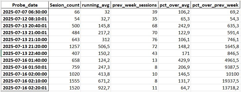
print("Anomalies Detected:")
# Display the identified anomalies with context
print(anomalies[[
'Sesion_count',
'running_avg',
'prev_week_sessions',
'pct_over_avg',
'pct_over_prev_week'
]].round(1))Program detected following anomalies
Moving average in SQL
Read more Python for analysts most important datetime functions