Customer Retention Survival Analysis

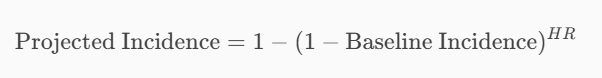
Customer Retention Survival Analysis. In survival analysis, the hazard ratio (HR) is the risk coefficient described the rate when event occurs in some conditions to the same events occurred under the control variable of interest. For example, in a clinical study of a treatment, the treated population may die at twice the rate of the control population. The hazard ratio (HR) would be 2, indicating a higher risk of death from the treatment applied to the population. To illustrate how hazard ratio is linked to projected risk let’s take to account a population where the incidence of some disease is 10% in selected age group (eg: Dementia), a hazard ratio of 4.42 results in an expected incidence of 37.3%. After some example we process Customer Retention Survival Analysis.

The hazard ratio is a measure of how often a particular event happens in one group compared to another over time. An HR of 2 means the event happens twice as often in the treatment group as in the control group.

Calculating Projected Incidence

To calculate the projected incidence percentage, you can use the following formula:

Here’s a step-by-step breakdown:

1. Baseline Incidence: This is the initial incidence rate in the control group. For example, if the baseline incidence is 10%, it means 10% of the control group experiences the event.
2. Hazard Ratio (HR): This is the ratio of the hazard rates between the treatment and control groups.

Let’s use your example where the baseline incidence is 10% (0.10) and the HR is 4.42.

1. Baseline Incidence: 0.10
2. HR: 4.42

Using the formula:

First, calculate ( (1 – 0.10) ): 0.90, Next, raise 0.90 to the power of 4.42: 0.90^{4.42} =\approx 0.627

Finally, subtract this result from 1: Projected Incidence = 1 – 0.627 = \approx 0.373 (37,3%)

In this example, a baseline incidence of 10% with an HR of 4.42 results in a projected incidence of 37.3%. This means that under the treatment condition, the incidence of the event (e.g., disease) is expected to increase to 37.3%.

COVID case

• Without treatment (control group): 80% of death (0.80)
• With vaccination (treatment group): 15% of death (0.15)

The HR is calculated as the ratio of the hazard rates between the treatment group and the control group. In this case, the treatment group is the vaccinated group, and the control group is the unvaccinated group.

So, the correct calculation is: HR = {0.15} / {0.80} = 0.1875

An HR of 0.1875 means that the risk of death after vaccination is about 18.75% of the risk of death without vaccination. This indicates a significant reduction in risk due to vaccination.

• HR > 1: Increased risk in the treatment group.
• HR < 1: Decreased risk in the treatment group.

In this case, since the HR is less than 1, it indicates that vaccination significantly reduces the risk of death from COVID-19.

Interpretation of HR

• HR > 1: The event (e.g., death, disease) is more likely to occur in the treatment group compared to the control group. This indicates an increased risk.
• HR < 1: The event is less likely to occur in the treatment group compared to the control group. This indicates a decreased risk.
• HR = 1: The event is equally likely to occur in both groups, indicating no difference in risk.

1. Increased Risk: If the HR is 2, the event is twice as likely to occur in the treatment group compared to the control group.
2. Decreased Risk: If the HR is 0.5, the event is half as likely to occur in the treatment group compared to the control group.

Always Positive

Since the HR is a ratio of two positive hazard rates, it will always be a positive number. Negative hazard ratios do not make sense in this context because hazard rates (which represent probabilities) cannot be negative.

Hazard ratios differ from relative risks (RRs) and odds ratios (ORs) in that RRs and ORs are cumulative over an entire study, using a defined endpoint, while HRs represent instantaneous risk over the study time period, or some subset thereof. Hazard ratios suffer somewhat less from selection bias with respect to the endpoints chosen and can indicate risks that happen before the endpoint.

Customer Retention Survival Analysis

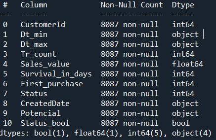
if we have data like this we can calculate Kaplan–Meier estimator.

The Kaplan–Meier estimator is a non-parametric statistic used to estimate the survival function from lifetime data. In medical research, it is often used to measure the fraction of patients living for a certain amount of time after treatment. In case of customer acquisition and then retention for revenue generation is the time from the moment of acquiring the customer to the moment the customer left the company. Other fields, Kaplan–Meier estimators may be used to measure the length of time customer remain passive before first purchase or passive after some marketing motivation has been applied. In similar way, the time-to-failure of machine parts, or how long fleshy fruits remain on plants. Can be also used to Customer Retention Survival Analysis.

The estimator is named after Edward L. Kaplan and Paul Meier, who each submitted similar manuscripts to the Journal of the American Statistical Association. The journal editor, John Tukey, convinced them to combine their work into one paper, which has been cited more than 34,000 times since its publication in 1958. Read more in Wikipedia.

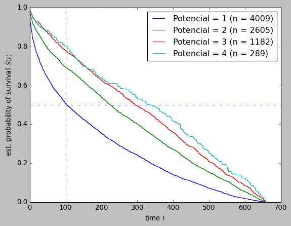
for p in sorted([x for x in df_cust["Potencial"].unique() if x>'0']) :
    mask_treat = df_cust["Potencial"] == p
    time_treatment, survival_prob_treatment, conf_int = kaplan_meier_estimator(
        df_cust["Status_bool"][mask_treat],
        df_cust["Survival_in_days"][mask_treat],
        conf_type="log-log",
    )

    plt.step(time_treatment, survival_prob_treatment, where="post", linewidth=1,
             label=f"Potencial = {p} (n = {mask_treat.sum()})")
    #plt.fill_between(time_treatment, conf_int[0], conf_int[1], alpha=0.25, step="post")


# Adding vertical and horizontal lines
plt.axvline(x=100, color='red', linestyle='--', linewidth=0.5) # Vertical line at x=10
plt.axhline(y=0.5, color='blue', linestyle='--', linewidth=0.5) # Horizontal line at y=0.5

plt.ylim(0, 1)
plt.ylabel(r"est. probability of survival $\hat{S}(t)$")
plt.xlabel("time $t$")
plt.legend(loc="best")

You can read abut customer churn prevention here Customer churn and here Strategies for customer retention.

What is Customer Churn?

The customer churn analysis can be defined as analytical work carried out on the possibility of a
customer leaving a product or service. In its simplest definition, it means that customers are
abandoned to choose the company because of competition. The purpose is to identify this
situation before leaving the customer’s product or service, and then to carry out some
preventive actions.

Importance of Churn Analysis

It is particularly important in the calculations of a business in sectors such as insurance,
telecommunications or banking, which is a subscription-based income model. According to
researchers, winning new customers in today’s competitive conditions is up to 10 times costlier
than retaining existing customers. Many parameters such as the costs, profitability, size, investment
capacity, cash flow of the enterprises depends on the number of customers and therefore the
loyalty of the customers.